BBT045: Sequencing Technologies Tutorial

Author: Vi Varga (Adapted from Filip Buric (adapted from Rui Pereira))

Last updated: 04.02.2025

Tutorial Overview

• Working with Jupyter Notebooks to construct reproducible procedures
• Running sequence processing software from the command line
• Running sequence processing software from wrapper Python modules
• Inspecting different output formats

Initial setup: Working environment and Data

The beginning of this Notebook includes information on setting up a conda environment under the "Working environment" heading. As you will be working on Vera, you will not be following those procedures! They are included only for reference, both as something you can look back at if/when you need to create and manage a conda environment yourself, as well as for you to be able to see my process, for how I went about setting up this Notebook. You can also download a copy of this Notebook from here for your own computer.

The notebook will serve as both a rudimentary pipeline and final (reproducible) report.

Directory and data setup

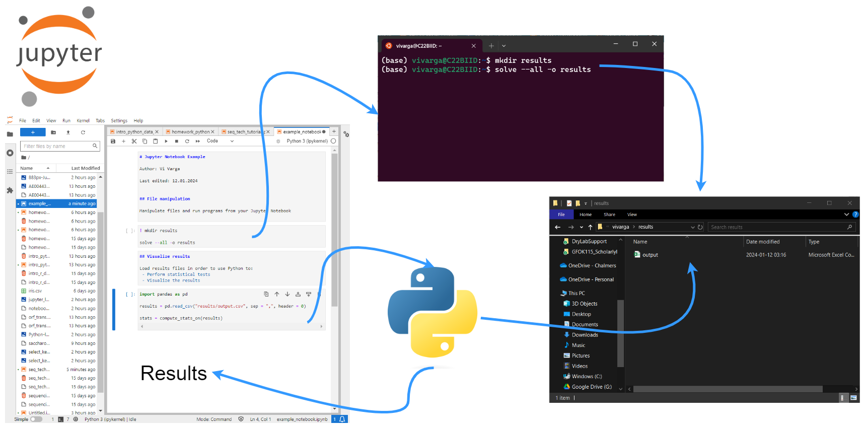
We will be working in Jupyter Lab and primarily writing the commands in this Jupyter Notebook. However, the first commands in this section are easier if you run them from the terminal. (Note that depending on how you have things set up on your computer, you may have access to a Unix terminal within Jupyter Lab. Simply do: "File" → "New" → "Terminal" and a terminal will open in a new tab in Jupyter Lab.)

Please create a directory for this tutorial in your home directory and inside there copy the starter notebook from my directory. To do this run the following commands in the terminal after logging on to the server:

cd
mkdir 
cd NGS_Tutorial
wget https://bengtssonpalme.github.io/MPBIO-BBT045-2025/seq_tech/seq_tech_tutorial_py.ipynb
###
# optionally, if you want the images to show up properly
cp -r /cephyr/NOBACKUP/groups/bbt045_2025/Resources/SeqTech/img/ .

Now fetch a copy of the data we will be using:

cp /cephyr/NOBACKUP/groups/bbt045_2025/Resources/SeqTech/data.zip .
# and now decompress the .zip file
unzip data.zip
# and clean up
rm -r __MACOSX/
# this directory is an artifact of the .zip file creation process
# it's unnecessary, so it can be deleted

Also copy over the runtime environment file you will need:

cp /cephyr/NOBACKUP/groups/bbt045_2025/Resources/SeqTech/seq-tech-jupyter.sh ~/portal/jupyter/

To nicely see the contents of (small) directories, you can use the tree program:

tree data

You can also run ls * (which works on any system).

Then create a results directory:

mkdir results

Working environment

Background

If you wish to create and use your own conda environments locally, on your own computer, you first need to install conda. See instructions here. Note that Vera does not like its users to create and use conda environments. This is because conda environments require a lot of files. Instead, all programs not already installed on Vera should be run from containers.

It's standard practice to create a new conda environment for each project. This is because each project may require a number of different software packages, with certain versions. Even if these requirements are very similar between the projects, even small differences may topple the house of cards that is the software ecosystem. This is officially referred to as "dependency hell" and can cause you more than a little frustration (to put it mildly).

Conda can fetch packages from many different sources (aka "channels"). For bioinformatics purposes, usually the most important are the Bioconda channel and the general-purpose conda-forge channel ("defaults" is given first to give it top priority when searching for packages).

You can add the channels by running the following in your Unix terminal (not in your Jupyter Notebook):

# adding conda channels
conda config --add channels defaults
conda config --add channels bioconda
conda config --add channels conda-forge

Setting up our environment

Once conda has been set up properly, the user can proceed to ceate and activate new environments. Here, I'll demonstrate how I did that for this exercise.

The conda create command creates new environments, the option --name (or -n) specifies the name of your new environment and the option -y lets conda know that you answer "yes" to all prompts. Without -y you will have to manually type in "yes" or "y" when prompted.

The command conda activate activates the environment within the current code chunk and only the current code chunk. Which means that within every code chunk that we want to use our environment we need to first run conda activate <environment_name>.

You could create and activate the conda environment used for this exercise by running the following in your Unix terminal (not in your Jupyter Notebook):

conda create --name sequencing -y
# you can activate the environment by running: 
conda activate sequencing

Installing relevant software

Now we can install the software needed for this exercise. We want to install the software into the new environment so we first activate the environment with conda activate. The command conda install will install the packages that you specify. You can specify multiple packages at a time by separating them with spaces. This step will also ask for confirmation if we do not specify the -y option.

Later on/in real life, it's good to to examine what changes are made when installing new packages. You can easily view all the packages installed in an environment by running conda list once the environment is activated.

Make sure you activate your environment prior to beginning software installation! Uninstalling software packages from the base conda environment is not an easy process.

While doing the installations, I ran the following lines of code from my Unix terminal:

conda activate sequencing
# conda install gsl==2.5 samtools bowtie2 breseq abyss bcftools wgsim emboss tree ncurses -y
# you can often install all packages in a conda environment as shown above
# however in this case, it's actually quicker to run multiple commands: 
conda install gsl==2.5
# this is necessary to prevent a dependency issue with bcftools
# ref: https://www.biostars.org/p/9480029/#9573995
conda install -c bioconda samtools
conda install -c bioconda bowtie2 
conda install -c bioconda breseq 
conda install -c bioconda abyss 
conda install -c bioconda bcftools 
conda install -c bioconda wgsim 
conda install -c bioconda emboss 
conda install tree
conda install -c conda-forge ncurses
# otherwise ncurses may install without a version number, which will cause samtools to raise an error
# ref: https://stackoverflow.com/questions/72103046/libtinfo-so-6-no-version-information-available-message-using-conda-environment
# and install a few python libraries
conda install pandas seaborn

It's later possible to inspect the installed packages with:

conda activate sequencing
conda list

Running conda in Jupyter Notebooks

Because Jupyter is packaged within an Anaconda installation, you should be able to run conda commands directly from this Jupyter Notebook with just a little modification. Simply install the IPython kernel in any environment you wish to use in Jupyter Notebooks, and the nb_conda_kernels program in your base conda environment.

PLEASE NOTE!!! Enable the creation of a kernel only after you have installed all of the programs you intend to install in your environment! Starting with the ipykernel installation can raise errors that will prevent you from installing the programs you are actually going to use in your environment!

# do this inside of your working conda environment, not in the base environment
conda install ipykernel

Now create a kernel for the conda environment, by running the following in that same Unix terminal:

# you can run this from the base conda environment
python -m ipykernel install --user --name=sequencing
# this should return something like: 
# Installed kernelspec sequencing in /home/vivarga/.local/share/jupyter/kernels/sequencing

For more information, check out this website.

Once you have installed the above in your environment, you also need to install the nb_conda_kernels program in your base conda environment:

# in base conda environment
conda install conda-forge::nb_conda_kernels
# ref: https://stackoverflow.com/questions/39604271/conda-environments-not-showing-up-in-jupyter-notebook/56409235#56409235

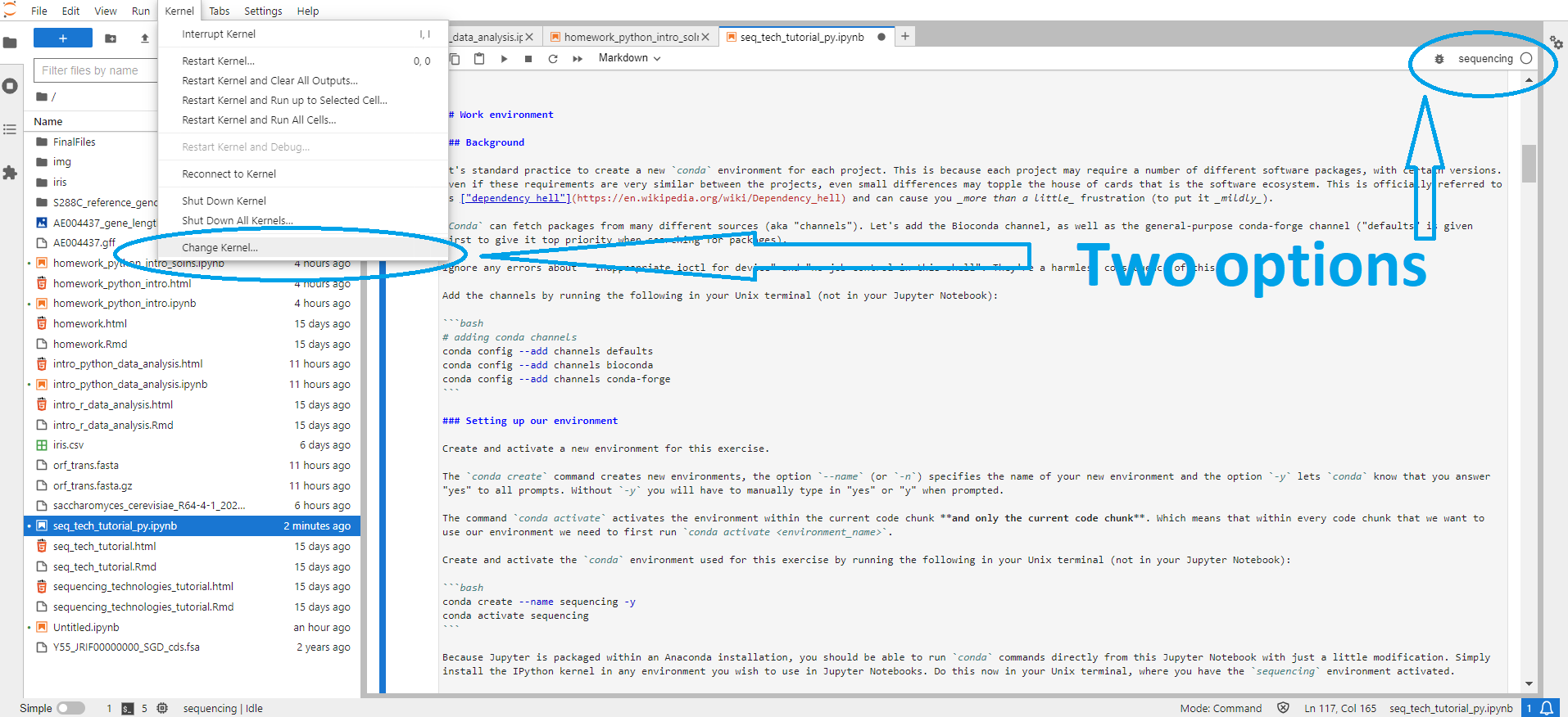
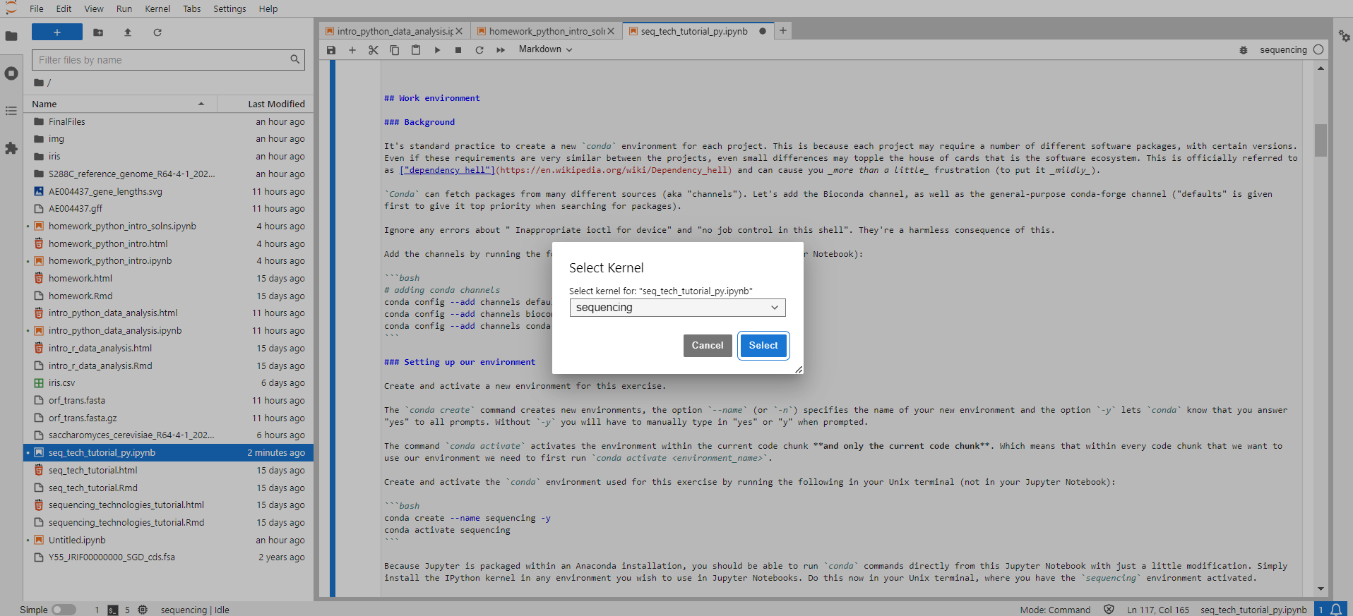
If you were following along because you want to try running this Notebook on your local computer (i.e., not on Vera), you should now be able to activate the sequencing conda environment within this Jupyter Notebook, by selecting the Python [conda env:sequencing] kernel within Jupyter Lab. Since you will be working within a kernel made from your conda environment, there will be no need to run conda activate sequencing in any of the cells in this Notebook. (There should also be a sequencing kernel, but you likely won't be able to run programs installed in the environment using this kernel.) This can be done either from the kernel display at the top right side of the Jupyter Lab screen, or via "Kernel" → "Change Kernel..." → select the kernel of choice

Compiling software into a container

In our case, we will be running Jupyter from a container on Vera, rather than directly from the command line. This is because we need a lot of software that doesn't come packaged with Python modules.

The container we will be using is available in the /cephyr/NOBACKUP/groups/bbt045_2025/Containers/ directory. It was created as is shown below:

# first, export the conda environment to a YAML file
conda env export -n sequencing > sequencing.yml
# build the container using Apptainer
apptainer build --build-arg ENV_FILE=sequencing.yml conda-sequencing.sif conda_environment_args_ubuntu.def

Running Jupyter from Vera OnDemand

This exercise is intended to be run similarly to how you ran the Python tutorial, using Vera OnDemand.

In order to ensure you start off correctly, please ensure the following:

• You have created your NGS_Tutorial/ directory and have downloaded this Jupyter Notebook into it
• You have copied all relevant files from the /cephyr/NOBACKUP/groups/bbt045_2025/Resources/SeqTech/ directory, particularly the data.zip file
• You have placed your copied the seq-tech-jupyter.sh file from the above directory to your local ~/portal/jupyter/ directory

If all of the above are true, set the path to your NGS_Tutorial/ directory as your working directory and the seq-tech-jupyter.sh script as your runtime, and launch Jupyter via Vera OnDemand. Remember to increase the default time requested to 3-4 hours, and ideally select an ICELAKE core, as the default SKYLAKE core may not function correctly.

Note that many of the commands in this Jupyter Notebook will raise the following error: "/usr/share/lmod/lmod/init/bash: line 25: /usr/share/lmod/lmod/libexec/addto: cannot execute: required file not found". Please just ignore it, as it is harmless - your commands will still run, regardless of this error being reported back to you. It is an artifact of the program containerization process.

Exercise 1: Alignment

We'll be aligning sequencing data against the reference genome of a Varicella virus.

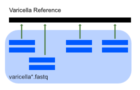
This mainly involves using bowtie2 to align short-read sequencing data to the reference genome and samtools to post-process and visualize the result:

Raw data files:

• Varicella reference genome: data/ref/varicella.gb
• Sequencing files: data/seq/varicella1.fastq, data/seq/varicella2.fastq

You can run the commands in the terminal directly to test them out, but they should be included (in order) in the Jupyter Notebook, so copy the code chunks and run the chunk from the notebook. The next code block demonstrates how to run bash commands from a Jupyter Notebook.

Protocol

Step 1: Init

Create a separate results directory, using either the command line, or your Jupyter Notebook. In your bash terminal, you can run:

mkdir results/exercise1

Alternately, you can run the folloing directly from your Jupyter Notebook. (Note the "! " at the start of the line; this tells Jupyter to execute the commands on that line on the command line, rather than in Python.)

# run bash commands from Jupyter Notebook with an ! at the start of the line
! mkdir -p results/exercise1
# -p also makes the parent directories
# so this command will work even if you forgot to make the results/ directory earlier

Step 2: Preprocess

bowtie2 requires an index file for the reference sequence. This index can only be constructed from a FASTA file but it's common practice to find reference genomes in GenBank (GFF3) format.

Convert varicella.gb to FASTA using the seqret converter from the EMBOSS package, then build the bowtie index accordingly.

(Computation time: seconds)

# Convert GFF3 > FASTA
! seqret -sequence data/ref/varicella.gb -feature -fformat gff3 -osformat fasta data/ref/varicella.fasta

# This file is outptut by seqret in the current directory (because bad design)
# So we move it where it belongs
! mv varicella.gff data/ref/

# Document how the FASTA file was created
! touch data/ref/README.txt
! echo "vaircella.fasta converted from GFF as:" > data/ref/README.txt
! echo "seqret -sequence data/ref/varicella.gb -feature -fformat gff3 -osformat fasta data/ref/varicella.fasta" >> data/ref/README.txt

# Save index files in own directory
! mkdir results/exercise1/bowtie_index
# Build the bowtie2 index
! bowtie2-build -f data/ref/varicella.fasta results/exercise1/bowtie_index/varicella

Step 3: Align sequences to reference

Align the sequencing data to the reference genome using bowtie2. This will create the file varicella.sam. The \ symbol simply breaks the command across multiple lines for readability.

(Computation time: 1 min)

! mkdir results/exercise1/alignment
! bowtie2 -x results/exercise1/bowtie_index/varicella -1 data/seq/varicella1.fastq -2 data/seq/varicella2.fastq -S results/exercise1/alignment/varicella.sam

Step 4: Convert alignment to binary format

To make reading the alignment info easier for the computer, convert the sequence alignment map (SAM) file to binary alignment map (BAM) using the samtools view command:

(Computation time: seconds)

! samtools view -b -S -o results/exercise1/alignment/varicella.bam results/exercise1/alignment/varicella.sam

Step 5: Optimize alignment (pt 1)

To optimize the lookup in the alignment map, sort the BAM file using samtools sort command. This will create the file varicella.sorted.bam

(Computation time: seconds)

! samtools sort results/exercise1/alignment/varicella.bam -o results/exercise1/alignment/varicella.sorted.bam

Step 6: Optimize alignment (pt 2)

To speed up reading the BAM file even more, index the sorted BAM file using samtools index command:

(Computation time: seconds)

This will create a BAI file called results/exercise1/alignment/varicella.sorted.bam.bai

! samtools index results/exercise1/alignment/varicella.sorted.bam

Step 7: Calculate alignment coverage

Calculate the average coverage of the alignment using the samtools depth command and the Unix awk text processor to extract the values of interest:

(Computation time: 1s)

Output should be:

Answer:

`Average = 199.775`

! samtools depth results/exercise1/alignment/varicella.sorted.bam | awk '{sum+=$3} END {print "Average = ", sum/124884}'

Question

Use the samtools depth command to extract coverage info and create a coverage map of the genome (position vs. coverage). Read the help for the tool with samtools help depth. The output format is described at the end of the help.

! samtools depth results/exercise1/alignment/varicella.sorted.bam > results/exercise1/alignment/coverage.tsv

Plot the result with Python:

# load necessary modules
import pandas as pd
import seaborn as sns
import matplotlib.pyplot as plt
import warnings # module to manage warnings
warnings.simplefilter(action='ignore', category=FutureWarning) # prevent Python from warning of future feature deprecation

# import data into Pandas dataframe
alignment_coverage_df = pd.read_csv('results/exercise1/alignment/coverage.tsv', sep = '\t', names = ["reference_name", "position", "coverage_depth"])

# create histogram of data
alignment_coverage_plot = sns.histplot(data = alignment_coverage_df, x = "coverage_depth")
# next add labels to the axes & a title
alignment_coverage_plot.set_title('Alignment Coverage')
alignment_coverage_plot.set_ylabel('Counts')
alignment_coverage_plot.set_xlabel('Alignment coverage depth')

# visualize the plot
alignment_coverage_plot

Exercise 2: Finding Mutations with SAMtools

We now look at a second set of sequencing data, with mutations (data/seq/varicella_mut1.fastq and data/seq/varicella_mut1.fastq)

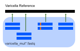
We'll still be using bowtie2 and samtools to perform these tasks, however we'll be structuring all the steps in to one script.

This approach has the great advantage that we don't need to copy-paste all we did above just to change the name of the input files. That's cumbersome and very error-prone. Instead we just need to change the file name at one location.

Protocol

Step 1: Align sequences to reference

Create a sorted and indexed BAM file using the code below, which encapsulates steps 2-6 from Exercise 1 (except for the GFF > FASTA conversion).

Tip: Run ls -l data/* or tree data if you forget what files you're working on.

The workflow will also create results/exercise2 for you.

(Computation time: 5 minutes)

Note that here I've used %%bash at the start of the cell; this is part of IPython's "cell magics". When you start a code cell with %%, you can transform the entire cell into a different language, rather than only transforming a single line. So for example, you could do %%R to transform a regular Jupyter Notebook code cell (which runs Python by default) into an R code cell.

%%bash

DATA_DIR=data/seq
RESULT_DIR=results/exercise2

REFERENCE_GENOME=data/ref/varicella.fasta
READS_1=$DATA_DIR/varicella_mut1.fastq
READS_2=$DATA_DIR/varicella_mut2.fastq


BOWTIE_INDEX_DIR=$RESULT_DIR/bowtie_index
ALIGNMENT_DIR=$RESULT_DIR/alignment

# Make all directories
mkdir $RESULT_DIR
mkdir $BOWTIE_INDEX_DIR
mkdir $ALIGNMENT_DIR

# Build the bowtie2 index
bowtie2-build -f $REFERENCE_GENOME $BOWTIE_INDEX_DIR/varicella


bowtie2 -x $BOWTIE_INDEX_DIR/varicella -1 $READS_1 -2 $READS_2 -S $ALIGNMENT_DIR/varicella_mut.sam

samtools view -b -S -o $ALIGNMENT_DIR/varicella_mut.bam $ALIGNMENT_DIR/varicella_mut.sam
    
samtools sort $ALIGNMENT_DIR/varicella_mut.bam -o $ALIGNMENT_DIR/varicella_mut.sorted.bam
    
samtools index $ALIGNMENT_DIR/varicella_mut.sorted.bam

Step 2: Identify point mutations

Use the samtools mpileup command to identify genomic variants (aka single nucleotide variants, SNVs) in the alignment. This will create the file varicella_variants.bcf

! bcftools mpileup -f data/ref/varicella.fasta results/exercise2/alignment/varicella_mut.sorted.bam -O u > results/exercise2/varicella_variants.bcf

Step 3: Inspect mutations (pt 1)

Use bcftools call command to convert the binary call format (BCF) to (human-readable) variant call format (VCF). This will create the file varicella_variants.vcf

! bcftools call -c -v results/exercise2/varicella_variants.bcf > results/exercise2/varicella_variants.vcf

If you wish to inspect it, run less -S results/exercise2/varicella_variants.vcf.

The file contains quite a lot of information, which we'll use later on. See https://en.wikipedia.org/wiki/Variant_Call_Format for more info.

Step 4: Inspect mutations (pt 2)

Visualize the mutation detected on site 77985 using the samtools tview command.

For this, you only need the BAM file. Remember that this files stores mutant-to-reference alignment information. VCF (and BCF) contain only the information needed for some downstream tasks.

This is an interactive command so run it in the terminal:

# note that when opening a terminal in Jupyter on Vera, you may not be located in your working directory
# run `pwd` and then navigate to your NGS_Tutorial/ working directory
# only then run the following command:
samtools tview results/exercise2/alignment/varicella_mut.sorted.bam data/ref/varicella.fasta -p NC_001348:77985

Questions

Q1

Inspect the VCF file columns using the Unix command chain:

# note that this command is also interactive - run it in the terminal
grep -v "^#"  results/exercise2/varicella_variants.vcf | column -t | less -S

(Chain: Filter out header | align columns | show on screen)

How can you interpret the PHRED score values in the last column? See the VCF specifications (Section 5)

Are all mutations homozygous? Should you expect any heterozygous mutations in this case?

Q2

What assumption does samtools mpileup make about the model of genetic mutations? (Try running bcftools mpileup for help and scroll down.)

Is this model appropriate for a virus?

Answer:

samtools mpileup assumes the data originates from a diploid organism and models mutations based on the existence of two similar copies of the same sequence. Since viruses only have one copy of the genome, this model is not correct and it is not possible for a single genomic position to have two different bases.

Q3

Use samtools mpileup to inspect the site 73233. What is the frequency of each base on this site?

Run the command below and see Pileup format

! samtools mpileup -r NC_001348:73233-73233 -f data/ref/varicella.fasta results/exercise2/alignment/varicella_mut.sorted.bam

Answer:

87 T, 1 A, 2 G

Exercise 3: Finding Mutations with breseq

Using the breseq pipeline to compute the mutations present in the mutant strain in comparison to the reference sequence provided for the varicella virus.

Protocol

Step 1: Init

Create the results directory for this exercise:

! mkdir results/exercise3

Step 2: Run

(Computation time: 5-10 minutes)

Run breseq

! breseq -j 1 -o results/exercise3 -r data/ref/varicella.gb data/seq/varicella_mut*.fastq

Questions

Q1

Open the index.html file in the results/exercise3/output folder and compare the mutations detected to those identified in Exercise 2.

Answer:

One mutation is missing in breseq

Q2

Use the breseq bam2aln command to investigate the missing mutations

Answer:

`breseq bam2aln -f data/ref/varicella.fasta -b results/exercise2/alignment/varicella_mut.sorted.bam -r NC_001348:117699-117699 -o results/exercise3/missing_mutations.html`

Now open the output results/exercise3/missing_mutations.html with Jupyter Lab.

Breseq missed this mutation in the output table.

Q3

Open the results/exercise3/output/summary.html file and find the mean coverage of the alignment.

Explore the results directory in ourder to find and take a look at the coverage plot.

Exercise 4: De novo genome assembly

So far we've been using a reference genome to align reads to it. When one is not available, the genome has to be assembled de novo from the reads. Here, we'll be using the abyss assembler with reads from the dumas strain of the varicella virus.

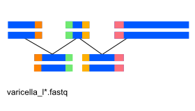
Sequencing files from dumas strain: data/varicella_l1.fastq, data/varicella_l2.fastq

Protocol

Step 1: Init

! mkdir results/exercise4

Step 1: Assembly

Assemble the reads provided into a genome using abyss-pe for k=128

(Computation time: 5 minutes)

! abyss-pe name=varicella k=100 B=8K s=150 --directory=results/exercise4 in='../../data/seq/varicella_l1.fastq ../../data/seq/varicella_l2.fastq'

Questions

Q1

How many unitigs, contigs and scaffolds were assembled?

Hint: less varicella-stats.md

Answer: Should be around: 87, 90, 62

Q2

How big is the largest scaffold?

Answer: 1000

Q3

What do you think, is this a good quality assembly? Hint: take a look through the messages printed to your screen!

Answer: Not really. Part way through, this warning is given: "warning: the seed-length should be at least twice k: k=100, s=150" The truth is, that I had to specifically modify the command in order to force it to work. This dataset doesn't produce a good assembly!

Q4

Use NCBI nucleotide blast (https://blast.ncbi.nlm.nih.gov/Blast.cgi) to find similar sequences to the scaffolds obtained.

What is the most similar sequence obtained?